Digitalizing GPX Points or How to Track Vehicles With GraphHopper

Recently I was asked again if I know a method, or even better a tool, which makes GPX points more align to the existing streets in OpenStreetMap. E.g. currently in Mapillary all recorded streets are not really smooth and digitalized if you look at them in detail. GraphHopper cannot do this out of the box but provides a toolchain which will make this digitalization easier.

Update: this is now open source.

Map Matching

The necessary process before an import would be Map Matching. Quoting (my own words ;)) from Wikipedia:

Map matching is the process of associating a sorted list of user or vehicle positions to the road network on a digital map. The main purposes are to track vehicles, analyze traffic flow and finding the start point of the driving directions.

Or as a picture:

I’m explaining in this blog post the simple steps which can taken to implement something like this with a very simple method. This is not an invention by me, other papers suggesting a similar technique. Also we should use some open testing data additionally to the normal unit tests. Some wordings are necessary before we go deeper:

• A GPS point is a tuple or object which contains latitude, longitude (, elevation) at which position it was recorded.
• A GPX point is a tuple or object which contains latitude, longitude (, elevation) and the timestamp at which it was recorded. And a GPX list ist a list of GPX points.
• In the digital world of maps we need a data structure to handle the road network. This data structure is a graph where the junctions from real world are nodes and the streets between them are the edges.

The question is also why would we need a routing engine at all?

Because:

• firstly you don’t need to write the import process of OpenStreetMap and the closest edge lookup and probably some other tools necessary for map matching and
• secondly the routing process will fill gaps between larger distances of two GPX points, and will be able to guess those gaps depending on the vehicle and
• thirdly using a routing engine will make the outcome more realistic, e.g. avoiding going left and then returning the identical street to go further in the straight direction.
• Lastly with GraphHopper you’ll be easily able to provide such a procedure even for the world wide case as it stores everything very compact and can be used in-memory or on-disc.

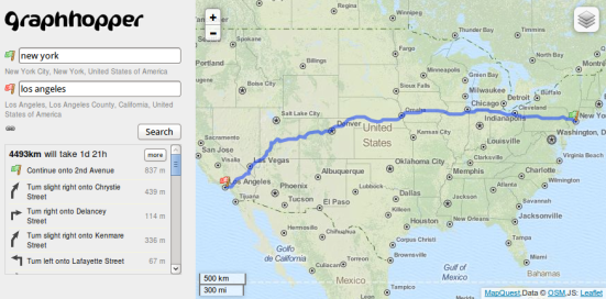
We start with an example:

All maps are from Lyrk and data is from OpenStreetMap contributors

In the left map you see the street parts highlighted where only the edges closest to the GPX points are selected. Whereas in the right map the most probable way was taken via a routing engine like GraphHopper.

The simple algorithm

The results for the map on the left side are easy to get, see the gist for example 1. For the map on the right side can try the following procedure explained in pseudocode here or see example 2 as gist for a more complete one:

1. Find 3 closest edges per GPX point
2. Associate every edge with a weighting, which is the distance from the edge to the point. The larger the distance the smaller is the probability that the best path goes through it.
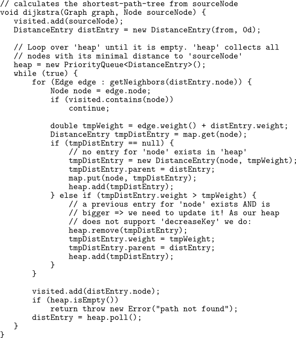
3. Find the best path from the first GPX point to the last, but take into account the weighting and therefor the distance to the GPX points
4. As a post-processing step you need to assign the GPX points to the resulting path, you can do so via the edge ids and to find the coordinates you can either use path.calcPoints or the lower level API ala edgeState.fetchWayGeometry.

This simple algorithm should work in the most cases and is very fast

The enhancements

There are two limitations of this simple algorithm:

• If there are loops in the GPX list, then the Dijkstra from step 3 will throw data away
• and it will happen that another route than the route marked with GPX points is taken. E.g. in the case if the GPX signal is not that frequent and the edge of one point is rather short, which means it will have a small influence on the overall weighting of the taken route.

The following improvements are possible

• You could do a simple workaround and cut the incoming GPX list when you detect a loop and feed those GPX-list-parts to the algorithm.
• Or find the best route not from start to end but ‘step by step’. For example from pointX to pointX+4, then pointX+4 to pointX+8 and so on, where you need to merge the results. To avoid suboptimal paths at the intersection (here pointX+4) you’ll need to ‘overlap’ the routes. So you will need to calculate the routes for pointX to pointX+4, then pointX+3 to pointX+7, …. instead. Merging will be more complex probably.
• A more complex solution could be to maintain a list of e.g. 3 alternative end-results. As you already get 3 edge candidates for every GPX point you can then try to find all routes between them. You could think that this will slow down the search a lot but with GraphHopper you can tweak e.g. the Dijkstra or DijkstraOneToMany algorithm to do this in an efficient manner. E.g. if you want to get the best result but you want to search from multiple destinations you can do: DijkstraBidirectionRef dijkstra = new DijkstraBidirectionRef(hopper.getGraph(), flagEncoder, weighting); dijkstra.initFrom(nodeFrom, distanceToPossibility1); dijkstra.initFrom(node, distanceToPossibility2); … dijkstra.initTo(nodeTo, distanceToEndPossibility1); dijkstra.initTo(nodeTo, distanceToEndPossibility2); …

There are lots of other problems which you’ll encounter, that is the ugly real life with GPS signal errors, tunnels and so on. One example problem is if you are tracking e.g. a truck waiting in front of traffic lights in a one way street. You’ll see several nearly identical GPX points but as they have an error associated they won’t be identical and it could happen that they go ‘backwards’ in the one-way which will result in an extra loop if use the ‘step-by-step’ variant of the shortest path calculation:

Languator: Language Detection for Local Queries

When you have an address lookup service like photon you need language detection for the short local queries like “Berlin Alexanderplatz” to e.g. apply a specific analysis chain. Of course German language is rather simple, but detecting if it is French or Italian etc is much more complex.

I tried the language-detection from google code. And although it has high precision for normal text, it is relative slow (creating the profile and querying) and not specific to local queries although short generic queries should work (e.g. Twitter data). Another problem is the complex and inflexible Java API as it uses lots of statics etc. E.g. the size of the n-grams is not configurable.

So I hacked together a new language detection called languator in Java specific for short local queries and fed it with OpenStreetMap data. E.g. I used the germany.pbf to create the German language profile and france.pbf for the French profile and so on. If you keep in mind that you have lots of foreign names for POI and street in every country the following error values are okayish and better than what I found from other tools:

English: 22.9%, German: 7%, French: 20%, Italian: 18.8%

Another good thing is that you can feed languator with these 4 countries in 20 minutes and create millions of queries from those countries which takes ~10 minutes, which is at least 2 times faster than the google code tool.

I invite you to beat my numbers: fork and have fun!

GraphHopper Maps 0.1 – High Performance and Customizable Routing in Java

Today we’re proud to announce the first stable release of GraphHopper! After over a year of busy development we finally reached version 0.1!

GraphHopper is a fast and Open Source road routing engine written in Java based on OpenStreetMap data. It handles the full planet on a 15GB server but is also scales down and can be embedded into your application! This means you’re able to run Germany-wide queries on Android with only 32MB in a few seconds. You can download the Android offline routing demo or have a look at our web instance which has world wide coverage for car, bike and pedestrian:

The trip to the current state of GraphHopper was rather stony as we had to start from scratch as there is currently no fast Java-based routing engine. What we’ve built is quite interesting as it shows that a Java application can be as fast as Bing or Google Maps (in 2011) and beats YOURS, MapQuest and Cloudmade according to the results outlined in a Blog post from Pascal and with tests against GraphHopper – although OSRM is still ahead. But how can a Java application be so fast? One important side is the used algorithm: Contraction Hierarchies – a ‘simple’ shortcutting technique to speed up especially lengthy queries. But even without this algorithm GraphHopper is fast which is a result of weeks of tuning for less memory consumption (yes, memory has something to do with speed), profiling and tweaking. But not only the routing is fast and memory efficient also the import process. And it should be easy to get started and modify GraphHopper to your needs.

Why would you use GraphHopper?

GraphHopper could be especially useful for more complicated or custom shortest/best path projects. E.g. if you need

• to embed GraphHopper or only parts of it directly within your Java application, which is easily possible due to the Apache 2 license.
• offline queries for your Android application
• highly customized routing (like horse routing – see below) where Google/Bing API calls aren’t sufficient or even possible
• many to many queries
• the shortest path tree(s) directly

… you should tell us on the mailing list what you need!

Community

GraphHopper is a young project but it makes great strides and it is already used in GPSies and in more places (cannot disclose all yet).

Last but not least I would like to thank NopMap for his work regarding OSM import and tuning, elevation data and much more! You can try out his horse routing prototype based on GraphHopper at the German WanderReitKarte.de (“trail riding map”)!

See the description on how you can contribute.

Have fun!

Preparing GraphHopper for its first release … (#Java #OpenStreetMap #Graph)

I’ve not blogged since a while but we are pushing Java road routing via GraphHopper to its first public release 0.1! We’re not finished yet, but have a first look and give us feedback here or in the mailing list (questions, bugs, …) so that we can release without big surprises in a few days or weeks 😉

Make Your Dijkstra Faster

Today I did a bit of research for GraphHopper and I stumbled over yet another minor trick which could speed up the execution of the Dijkstra algorithm. Let me shortly introduce this shortest path algorithm:

If you need the path (and not only the shortest path tree) you will give the method an additional toNode parameter and compare this to distEntry.node to break the loop. When it was found you need to recursivly extract the path from the last distEntry.parent reference.

So, what should we improve?

Regarding performance I’ve already included a Map to directly get the DistanceEntry from a node, otherwise you would need to search it in the PriorityQueue which is too slow. Also Wikipedias says that we could use a Fibonacci heap which are optimal to decrease the key (aka weight) but those are very complicated to implement and memory intensive.

It turned out that you can entirely avoid the ‘decrease key’ operation if you do a visited.contains check after polling from the queue. This makes your heap bigger but you can avoid the costly update operation and use simpler data structures. Read the full paper “Priority Queues and Dijkstra’s Algorithm”.

What else can we improve?

Now we can tune some data structures:

1. Make sure that you a traversing your graph with full speed. E.g. using just the graph in-memory without any persistence storage dependency could massivly improve performance. Also if you use node indices (pointing to an array) instead of node objects you can reduce memory consumption and e.g. use a BitSet instead of a set for the visited collection.
2. In case your heap is relative big (>1000 entries) like for multi-dimensional graphs and even for plane graphs then a cached version with 2 or more stages could give you a 30% boost. When you like more complicated and efficient solutions you could implement the probably faster sequence heap and others.
3. If you have a limited range of weights/keys you can try a TreeMap<Key, Set> which could speed up your code by roughly 10% if you heavily use the decreaseKey method.

For road networks and others you can apply A* which reduces the amount of visited nodes via guessing where the goal is – still the path is optimal IF the real path is longer than to what you guessed (e.g. use direct linear distance in road networks which is always smaller to the real distance):

PRESS ESC IF YOU GET NERVOUS 😉

Additionally if you accept some less optimal solutions you can apply heuristics like “don’t explore that much more nodes if you’r close the destination”.

If you don’t want less optimal paths and still want it faster you could

• use a bidirectional Dijkstra
• prepare your graph via ‘contraction hierarchies‘ which introduces several shortcuts and extremly reduces the number of visited nodes. It should also work for none-road networks too.

Running Shortest-Path Algorithms on the German Road Network within a 1.5GB JVM

Update: With changes introduced in January 2013 you only need 1GB – live demo!

In one of my last blog posts I wrote about memory efficient ways of coding Java. My conclusion was not a bright one for Java: “This time the simplicity of C++ easily beats Java, because in Java you need to operate on bits and bytes”. But I am still convinced that in nearly every other area Java is a good choice. Just some guys need to implement the dirty parts of memory efficient data structures and provide a nice API for the rest of the world. That’s what I had in mind with

GraphHopper

GraphHopper does not attack memory efficient data structures like Trove4j etc. Instead it’ll focus on spatial indices, routing algorithms and other “geo-graph” experiments. A road network can already be stored and you can execute Dijkstra, bidirectional Dijkstra, A* etc on it.

Months ago I took the opportunity and tried to import the full road network of Germany via OSM. It failed. I couldn’t make it working in the first days due to massive RAM usage of HashMaps for around 100 mio data points (only 33 mio are associated to roads though). Even using only trove4j brought no success. When using Neo4J the import worked, but it was very slow and when executing algorithms the memory consumption was too high when too many nodes where requested (long paths).

Then after days I created a memory mapped graph implementation in GraphHopper and it worked too. But the implementation is a bit tricky to understand, not thread safe (even not for two reading threads yet), slower compared to a pure in-memory solution. But even more important: the speed was not very predictable and very ugly to debug if off-heap memory got rare.

I’ve now created a ‘safe’ in-memory graph, which saves the data after import and reads once before it starts. At the moment this is read-thread-safe only, as full thread safety would be too slow and is not necessary (yet).

Now performance wise on this big network, well … I won’t talk about the speed of a normal Dijkstra, give me some more time to improve the speed up technics. For a smaller network you can see below that even for this simplistic approach (no edge-contraction or edge-reduction at all) the query time is under 150ms and will be under 100ms for bidirectional A* (w/o approximation!), I guess.

In order to perform realistic route queries on a road network we would like to satisfy two use cases:

1. Searching addresses (cities, streets etc)
2. Clicking directly on the map to create a route query

The first one is simple to solve and it is very unlikely to avoid tons of additional RAM. But we can solve it very easy with ElasticSearch or Lucene: just associate the cities, streets etc to the node ids of the graph.

The second use case requires more thinking because we want it memory efficient. A normal quad-tree is not a good choice as it requires too many references. Even for a few million data points it requires several dozens of MB in addition to the graph! E.g. 80MB for only 4 mio nodes.

The solution is to use a raster over the area – which can be a simple array addressed by spatial keys. And per quadrant (aka tile) we store one array index of the graph as entry point. (In fact this is a quad-tree of depth one!) Then when a click on the map happened, we can calculate the spatial key from this point (A), then get the entry point from the array and traverse the graph to get the point in the graph which is the closest one to point A. Here is an implementation, where only one problem remains (which is solved in the new index).

Unfair Comparison

In the last days, just for the sake of fun, I took Neo4J and ran my bidirectional Dijkstra with a small data set – unterfranken (1 mio nodes). GraphHopper is around 8 times faster and uses 5 times less RAM:

The lower the better – it is the mean time in seconds per run on this road network where two of the algorithms (BiDijkstraRef, BiDijkstra) are used. The number in brackets is the actually used memory in GB for the JVM. The lowest possible memory for GraphHopper was around 160MB, but only for the more memory friendly version (BiDikstra).

For all Neo4J-Bashers: this is not a fair comparison as GraphHopper is highly specialized and will only be usable for 2D networks (roads, public transport) and it is also does not have transaction support etc. as pointed out by Michael:

@timetabling gcr is a better cache from neo4j enterprise, and concurr. sync is not optional in a full ACID db, but your impl is a good test

— Michael Hunger (@mesirii) July 5, 2012

But we can learn that sometimes it is really worth the effort to create a specialized solution. The right tools for the right job.

Conclusion

Although it is not easy to create memory efficient solutions in Java, with GraphHopper it is possible to import (2.5GB) and use (1.5GB) a road network of the size of Germany on a normal sized machine. This makes it possible to process even large road networks on one machine and e.g. lets you run algorithms on even a single, small Amazon instance. If you reduce memory usage of your (routing) application you are also very likely to avoid garbage collection tuning.

There is still a lot room to optimize memory usage and especially speed, because there is a lot of research about road networks! You’re invited to fork & contribute!

Failed Experiment: Memory Efficient Spatial Hashtable

The Background of my Idea

The idea is to use a hash table for points (aka HashMap in Java) and try to implement neighbor searches. First of all you’ll need to understand what a spatial key is. Here you can read the details, but in short it is a binary Geohash where you avoid the memory inefficient base 32 representation.

Now that we have the spatial key, you can think about an array which is used to map from indices (like spatial keys) to values. This is the simplest representation of a spatial index as we don’t need to store the keys at all. But it is only memory efficient iff we would have no empty entries, which is very unlikely for clustered, real-world GIS-data.

If we would solve this with a normal hash table we encounter two problems:

• It is very unlikely that points in the same area come into the same hash bucket – making neighborhood searches slow i.e. O(n)
• It would be necessary to store the entire point – not only the associated value. Otherwise it would be impossible in case of a hash-collision to detect which point belongs to which value.

My idea is to use parts of the spatial key for the hashcode and avoid storing the entire key. It is implemented in Java (open source and available at GitHub).

As you can see we’re still using an array of buckets and a “somehow” converted spatial key to get

The Bucket Index

Let me explain the necessary bucket index in more detail (see picture above on the right).

We skip the beginning bits of every spatial key as it is  identical for an area a lot smaller than the world boundaries like Germany.

If we use the first part of the spatial key – in the picture identified as x, then the array is small enough. But with some real world data (also available as osm) this is not sufficient. Too many overflows would happen, some buckets would have several thousands entries! If we move the used part a bit to the right this gets a lot better e.g. for 4 entries per bucket we have a RMS error of about 2.

We now have a form of

A Hashtable & Quadtree Mixture

We can tune if our data structure behaves like a quad tree or a hash table. When moving the bits taken from spatial key to the left we get an quad tree-like characteristics. Taking the bits more from the right we get hash table-like characteristics.

This would be fine if we have massive data. But we need to make this approach practical also e.g. for only 2 mio data points. Because the part of the spatial key is only 19 bits long: if we assume 4 entries per bucket we come to approx. 2 mio (4 * 2^19 = 4 * 524 288). So the bucket index alone is too short. The solution to this problem is to do a bit-operation of the left and the right part of the spatial key:

bucketIndex = x ^ y

Further reduce memory consumption

Besides the fact that we now have some kind of a pointer-less or linear quad tree we can further reduce the memory footprint. We store only the required part (e.g. all bits except y) and not the full spatial key. For this it was necessary that our bit operation (or more generic “hashing scheme”) is reversible. Ie.: we can regain the full spatial key from only the bucket index and the stored part of the key. And in our case the x XOR y it reversible. In fact this memory reduction can be applied to any hashing procedure which fulfills this ‘reversible’ requirement.

Speed of Neighbor Queries is Bad

Neighborhood searches are very slow, slower than I expected. The naiv approach resulted in 60 seconds for a 10km search – 30 times slower as it would take to process all 2 mio entries. When tuning the overflow schema we are now a bit under 2 seconds. Still 10 times slower than a normal quad tree and as slow as processing all entries. The reason for why this storage is only good for get and put operations is that the same bucket needs to be parsed several times: as the same bucket index needs to be the home for several different locations – yeah, exactly as intended.

The good news are:

1. When I was moving the bucket-index-window a lot to the left it gets faster and faster, but took dozens of seconds to create the storage due to the heavy overflow number even for my small data set (2 mio). It could be improved a bit when applying different overflow strategies e.g. not using a linear overflow but skipping every two buckets or others.

2. Even in this state this idea can be used as a memory efficient spatial key-value storage without the neighbor search. E.g. you already have a graph of roads but you need an entrance like a HashMap<Point,NodeId> for it, then our data structure is an efficient hash table. Also doing a simple rectangular neighbor search should be fast: requesting only the 8 surrounding bounding boxes. Then no tree traversal is necessary and every box can be done with just a loop through the bucket array.

3. Another possibility is to use a small quadtree as an entry (mapping spatial keys to ids) for a 2D-graph. Then traversing this graph to find neighbors. This way I’ve finally chosen as I already needed a road-network for Dijkstra. So I only need additional 10MB for the small quadtree inex, see a possible next blog entry.

4. I’m not alone – you can take my idea and try implementing a more efficient neighbor searches yourself 🙂 !

Conclusion

In this post I’ve explained how to create a spatial hash table which is optimized in memory usage. This is achieved combining two ideas: using a hash table-alike data structure still ‘somehow suited’ for neighborhood searches and reducing the amount of memory while storing only parts of the hashkey. This second idea could be applied on every kind of hash table but only if the hashkey creation is reversible.

The ideas are implemented in Java for the GraphHopper project –  see the geohash package. Sadly the perfomance for neighbor searches is really bad. Which created a different solution in my mind (see point 3 of good news).

Outlook

In the literature similar data structures are called linear or pointer-less quad trees. After this experiment I come to the conclusion that the best way to implement a memory efficient spatial storage which is also able to perform fast neighbor queries could be a prefix quad tree. Still using pointers but storing two bits in very branch node and avoid those bits in the leaf nodes. Ongoing work for this is done currently in Spatial4J & Lucene 4.0 – actually without the use of spatial keys.

Tricks to Speed up Neighbor Searches of Quadtrees. #geo #spatial #java

In Java land there are at least two quadtree implementations which are not yet optimal, so I though I’ll post some possibilities to tune them. Some of those possibilities are already implemented in my GraphHopper project.

Quadtree

What is a quadtree? Wikipedia says: “A quadtree is a tree data structure in which each internal node has exactly four children.” And then you need some leaf nodes to actually store some data – e.g. points and associated values.

A quadtree is often used for fast neighbor searches of spatial data like points or lines. And a quadtree with points could work like the following: fill up a leaf node until its full (e.g. 8 entries), then create a branch node with 4 pointers (north-west, north-east, south-west, south-east) and decide where the leaf node entries should go depending of its location, in this process it could be necessary to create new branch nodes if all entries are too much clustered.

Now a simple neighbor search can be implemented recursively. Starting from the root node:

• If the current node is a leaf node check if the point is in the search area. If that is the case add it to the results
• If it is branch node check if one of the 4 sub-areas intersects with the search area. If a sub-node intersects then use that as current node and call this method recursively.

Trick 1 – Normalize the Distance

Searches are normally done with a point and a radius. To check if the current area of the quadrant intersects with the search area you need to calculate the distance using the Haversine formula. But you don’t need to calculate it every time in its entire complexity. E.g. you can avoid the following calculation:

R * 2 * Math.asin(Math.sqrt(a));

This is ok, if you have already normalized the radius of the search area via:

double tmp = Math.sin(dist / 2 / R);
return tmp * tmp;

Trick 2 – Use Smart Intersect Methods

The intersect method should fail fast. E.g. when you use again a circle as search area you should calculate only once the bounding box and check intersection of this with the quadrant area before applying the heavy intersect calculation with the Haversine formula:

public boolean intersect(BBox b) {
    // test top intersect
    if (lat > b.maxLat) {
        if (lon < b.minLon)
            return normDist(b.maxLat, b.minLon)  b.maxLon)
            return normDist(b.maxLat, b.maxLon)  0;
    }

    // test bottom intersect
    if (lat < b.minLat) {
        if (lon < b.minLon)
            return normDist(b.minLat, b.minLon)  b.maxLon)
            return normDist(b.minLat, b.maxLon)  0;
    }

    // test middle intersect
    if (lon < b.minLon)         return bbox.maxLon - b.minLon > 0;
    if (lon > b.maxLon)
        return b.maxLon - bbox.minLon > 0;
    return true;
}

Also be very sure you defined your bounding box properly once and for all. I’m using: minLon, maxLon followed by minLat which is south(!) and maxLat. Equally to EX_GeographicBoundingBox in the ISO 19115 standard see this discussion.

Trick 3 – Use Contains() and not only Intersect()

Now a less obvious trick. You could completely avoid intersect calls of quadrant areas which lay entirely in the search area. For this it is necessary to calculate fast if the search area fully contains the quadrant area or not. E.g. the method for a boudning box containing another bounding box would be:

class BBox {
  public boolean contains(BBox b) {
    return maxLat >= b.maxLat && minLat = b.maxLon && minLon   }
  ...
}

Similar for BBox.contains(Circle), Circle.contains(BBox) and Circle.contains(Circle).

Trick 4 – Sort In Time and not just Adding

Normally you want only 10 or less nearest neighbors and not all neighbours in a fixed distance. Especially for search engines like Lucene this should be favoured. For that you should use a priority queue to handle the ordering of the result. But not only of the leaf nodes – also when deciding which branch node should be processed next! See the paper Ranking in spatial databases for more information, where also a method for incremental neighbor search is described. This would make paging through the results very efficient.

Trick 5 – Use Branch Nodes with more than Four Children

Instead of branch nodes with 4 children you could use a less memory efficient but faster arrangement: use branch nodes with 16 child nodes. Or you could even decide on demand which branch node you should use – this can lead to partially big branch arrays where the quadtree is complete – making searching very efficient as then the sub-quadtree is a linear quadtree (see below).

Tricks for linear QuadTrees

Trick 6 – Avoid costly intersect methods

This only applies if you quadtree is a linear one ie. one where you can access the values by spatial keys (aka locational code). You’ll need to compute the spatial key of all four corners of your search area bounding box. Than compute the common bit-prefix of the points and start with that bit key instead from zero to traverse the quadtree. More details are available in the paper Speeding Up Construction of Quadtrees for Spatial Indexing  p.12.

Trick 7 – Bulk processing for linear Quadtrees

If you know that a quadrant is completely contained in a search area you can not only avoid further intersection calls, but also you can completely avoid branching and loop from quadrants bottom-left point to top-right. E.g. your are at key=1011 and you know the current quadrant node is contained in the search area. Then you can loop from the index “1011 000000..” to “1011 111111..”

Trick 8 – Store some Bits from the Point in Branch Nodes

For linear quadtrees you already encoded the point into spatial keys. Now you can use a radix tree to store the data memory efficient: some bits of the spatial key can be stored directly in the branch nodes. I’ve create also a different approach of a memory efficient spatial storage but as it turns out it is not that easy to handle when you need neighbor searches.

Conclusion

As you can see a lot time can go into tuning a quadtree. But at least the first tricks I mentioned should be used as they are easy and fast to apply and will make your quadtree significant faster.

Spatial Keys – Memory Efficient Geohashes

When you are operating on geographical data you can use latitude and longitude to specify a location somewhere on earth. To look up some associated information like we do in GraphHopper for the next street or if you want to do neighborhood searches you could create R-trees, quad-trees or similar spatial data structures to make them efficient. Some people are using Geohashes instead because then the neighborhood searches are relative easy to implement with simple database queries.

In some cases you’ll find binary representations of Geohashes – I named them spatial keys – in the literature I found a similar representation named locational code (Gargantini 1982) or QuadTiles at OpenStreetMap. A spatial key works like a Geohash but for the implementation a binary representation instead of one with characters is chosen:

At the first level (e.g. assume world boundaries) for the latitude we have to decide whether the point is at the northern (1) or southern (0) hemisphere. Then for the longitude we need to know wether it is in the west (0) or in the east (1) of the prime meridian resulting in 11 for the image below. Then for the next level we “step into” smaller boundaries (lat=0..90°,lon=0..+180°) and we do the same categorization resulting in a spatial key of 4 bits: 11 10

The encoding works in Java as follows:

long hash = 0;
double minLat = minLatI;
double maxLat = maxLatI;
double minLon = minLonI;
double maxLon = maxLonI;
int i = 0;
while (true) {
    if (minLat  midLat) {
            hash |= 1;
            minLat = midLat;
        } else
            maxLat = midLat;
    }

    hash <<= 1;
    if (minLon  midLon) {
            hash |= 1;
            minLon = midLon;
        } else
            maxLon = midLon;
    }

    i++;
    if (i < iterations)
        hash <<= 1;
    else
        break;
}
return hash;

When we have calculated 25 levels (50 bits) we are in the same range of float precision. The float precision is approx. 1m=40000km/2^25 assuming that for a lat,lon-float representation we use 3 digits before the comma and 5 digits after. Then a difference of 0.00001 (lat2-lat1) means 1m which can be easily calculated using the Haversine formula. So, with spatial keys we can either safe around 14 bits per point or we are a bit more precise for the same memory usage than using 2 floats.

I choose the definition Lat, Lon as it is more common for a spatial point, although it is against the mathematic point x,y.

Now that we have defined the spatial key we see that it has the same properties as a Geohash – e.g. reducing the length (“removing some bits on the right”) results in a broader matching region.

Additionally the order of the quadrants could be chosen differently – instead of the Z-curve (also known as Morton Code) you could use the Hilbert Curve:

But as you can see, this would make the implementation a bit more complicated and e.g. the orientation of the “U” order depends on previous levels –  but the neighborhood searches would be more efficient – this is also explained a bit in the paper Speeding Up Construction of Quadtrees for Spatial Indexing  p.8.

I decided to avoid that optimization. Let me know if you have some working code of SpatialKeyAlgo for it 🙂 ! It should be noted that there are other space filling curves like the ones from Peano or Sierpinsky.

One problem

while implementing this was to get the same point out of decode(encode(point)) again. The encoding/decoding schema needs to be “nearly bijective” – i.e. it should avoid rounding problems as good as possible. To illustrate where I got a problem assume that the point P (e.g. see the image above) is encoded to 1110 – so we already lost precision, when our point is now at the bottom left of the quadrant 1110. Now if we decode it back we loose again some precision due to normal double rounding errors. If we would encode that point again it could end up as 1001 – the point moved one quadrant to the right and one to the bottom! To avoid that, you need to define position of the point at the center of the quadrant while decoding. I implemented this simply by adding half of the quadrant width to the latitude and longitude. This makes the encoding/decoding stable even if there are minor rounding issues while decoding.

A nice property of the spatial key

is that one bounding box e.g. for the starting bits at level 6:

110011

goes from the bottom left point

110011 0000..

to the top-right point

110011 1111..

making it easy to request e.g. the surrounding bounding boxes of a point for every level.

Conclusion

As we have seen the spatial key is just a different representation of a Geohash with the same properties but uses a lot less memory. The next time you index Geohashes in your DB use a long value instead of a lengthy string.

In the next post you will learn how we can implement a memory efficient spatial data structure with the help of spatial keys. If you want to look at a normal quadtree implemented with spatial keys you can take a look right now at my GraphHopper project. With this quadtree neighborhood searches are approx. twice times slower than one with values for latitude and longitude due to the necessary encoding/decoding. Have a look into the performance comparison project.

Free Online Graph Theory Books and Resources

A link compilation of some Hackernews and Stackoverflow posts and a longish personal investigation.

• The DaMN book and its companion book
• Graph Theory with Applications, J.A. Bondy and U.S.R. Murty
• Graph Theory, Reinhard Diestel
• Graph Theory Tutorials
• Digraphs: Theory, Algorithms and Applications, 1st Edition
• Wikipedia – Graph Algorithms
• Algorithms and Complexity, Herbert S. Wilf
• Lecture notes Graphtheory by Tero Harju (Finland)
• Lecture notes Graphtheory by Keijo Ruohonen (Finland)
• Lessons at Math Cove
• Basics of Graphs

Google books

• Graph Theory with Application to Engineering and Computer Science, by Narsingh Deo
• A Course in Combinatorics

Chapters:

• Chapter 4. Algorithms, 4th Edition by Robert Sedgewick and Kevin Wayne – a nice explanation with Java examples and exercises
• Chapter 5. Graphs and graph algorithms
• Graph Search Algorithms in the Book “How to Think About Algorithms” from Jeff Edmonds
• Boost Docs – for C++ guys
• Chapter 7: Weighted Graphs

Visualizations

• Dijkstra & Co and some more Dijkstra
• A Star

None-free

• Introduction to Algorithms
• Graphentheorie by Clark and Holten
• Chapters from The Algorithm Design Manual, by Steven S. Skiena